GCP Cost Optimization Guide: Practical Strategies That Actually Reduce Your Bill

On GCP the biggest cost lever is usually BigQuery, not compute. On-demand BigQuery bills $6.25 per TiB scanned, so partition pruning and column pruning change the quantity the price multiplies. After that: take the Sustained Use Discount you already get automatically, buy resource-based Committed Use Discounts on your baseline at 37% for one year, and move fault-tolerant work to Spot VMs.

GCP’s pricing model differs from AWS and Azure in ways that change the order of the work. Sustained Use Discounts apply with no action. Committed Use Discounts need no upfront payment. And BigQuery’s per-query default can be either very cheap or very expensive depending entirely on how your analysts write SQL. Every figure below is us-central1 list price.

What are Sustained Use Discounts and who gets them?

GCP automatically applies Sustained Use Discounts (SUDs) to Compute Engine VMs that run for more than 25% of a billing month. No commitment, no action required, and the discount grows the longer an instance runs.

How SUDs scale on N1:

Usage in month	Share of on-demand price charged	Cumulative effective discount
0–25%	100%	0%
25–50%	80%	10%
50–75%	60%	20%
75–100%	40%	30%

For an n1-standard-4 running the whole month in us-central1, the on-demand price is $0.190/hr ($138.70/month). With SUDs applied automatically, the effective cost is about $97/month.

Which machine families miss out?

The maximum SUD is not the same everywhere, and several popular families get nothing at all.

• N1 tops out at 30% effective for a full month, as in the table above.
• N2, N2D and C2 top out at 20%. The brackets charge 100%, 86.78%, 73.3% and 60% of on-demand.
• E2, C2D, T2D, T2A, C3, C3D, C4 and N4 get no SUD. Neither do the accelerator-optimized A2 and G2 families.
• Custom machine types on N1 and N2 do qualify, contrary to a common misreading.

Two more constraints worth knowing: SUDs apply to self-serve billing accounts, and they do not stack with Committed Use Discounts. Neither AWS nor Azure has an equivalent automatic discount, so a GCP baseline is already lower before you optimize anything.

When should you buy a Committed Use Discount?

Buy one once your Compute Engine floor has been stable for a quarter. GCP now sells two kinds and they are not interchangeable.

Resource-based CUDs commit you to a number of vCPUs and GB of memory in a region, and pay the deepest discount. Flexible CUDs commit you to a dollar amount of spend and pay less for the extra freedom.

Commitment	1-year discount	3-year discount
Resource-based CUD	37%	55%
Flexible (spend-based) CUD	28%	46%

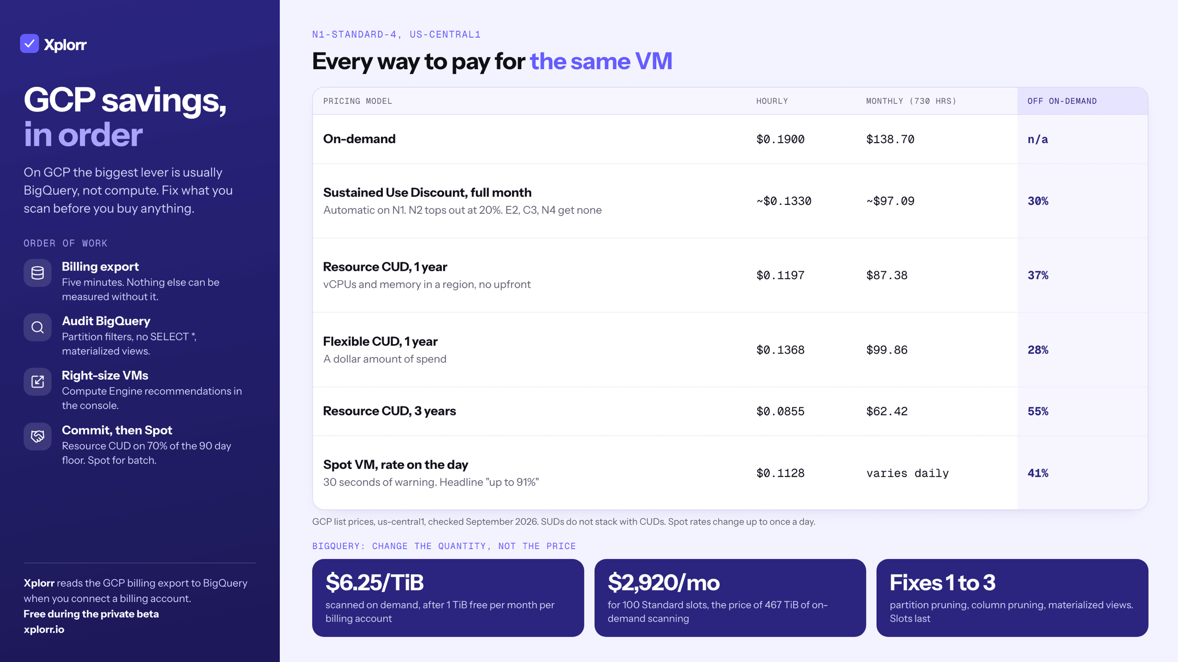
n1-standard-4 in us-central1, all models:

Pricing model	Hourly	Monthly (730 hrs)	Savings vs on-demand
On-demand	$0.1900	$138.70	n/a
With SUDs, full month	~$0.1330	~$97.09	30%
Resource CUD, 1-year	$0.1197	$87.38	37%
Flexible CUD, 1-year	$0.1368	$99.86	28%
Resource CUD, 3-year	$0.0855	$62.42	55%
Flexible CUD, 3-year	$0.1026	$74.90	46%

Prices checked September 2026, us-central1.

How do you size a CUD commitment?

Resource CUDs are not instance-based. You commit to vCPUs and GB of memory in a region, and GCP applies the discount across any eligible VM that uses them. You can change machine types, resize instances or redistribute workloads without losing the discount, as long as regional usage stays above the commitment.

Pull your floor from billing export:

SELECT
  DATE_TRUNC(usage_start_time, MONTH) as month,
  sku.description,
  SUM(usage.amount) as total_usage,
  usage.unit
FROM `project.dataset.gcp_billing_export_v1_XXXXXX`
WHERE service.description = 'Compute Engine'
  AND sku.description LIKE '%Core%'
  AND usage_start_time >= TIMESTAMP_SUB(CURRENT_TIMESTAMP(), INTERVAL 90 DAY)
GROUP BY 1, 2, 4
ORDER BY 1, 3 DESC

Look at your minimum monthly vCPU and memory usage and commit to 70–80% of that floor. Unlike AWS Reserved Instances, CUDs need no upfront payment, so the risk is a monthly bill you keep paying rather than capital already spent.

What do GCP Spot VMs actually cost?

Google publishes “discounts of up to 91%” for Spot VMs, but the ceiling is not the rate you get. Spot prices move up to once a day and vary by machine type and zone, so price the workload against today’s rate rather than the headline.

Instance	On-demand	Spot	Actual discount
n1-standard-4	$0.1900/hr	$0.1128/hr	41%
n1-standard-8	$0.3800/hr	$0.2255/hr	41%
n2-standard-4	$0.1942/hr	$0.1165/hr	40%

Prices checked September 2026, us-central1. Spot rates are recalculated by Google up to once per day.

Two practical notes. GCP reclaims a Spot VM with 30 seconds of warning, so your workload has to handle that. And Spot VMs have no maximum runtime, which is the main difference from the legacy Preemptible VMs they replaced: those were terminated after 24 hours no matter what.

Which workloads suit Spot VMs?

• CI/CD runners. Jenkins agents, GitHub Actions self-hosted runners, GitLab runners. A preempted build just restarts. Ten n1-standard-8 build agents at on-demand list are 10 x 0.38 x 730 = $2,774/month; at the current Spot rate they are 10 x 0.2255 x 730 = $1,646/month, so $1,128/month less.
• Batch processing. ETL jobs, video transcoding, image processing. Break work into small units, checkpoint progress, retry failed units. Apache Beam, Dataflow and Kubernetes Jobs all handle this natively.
• Data pipeline workers. Spark executors on Dataproc, Flink task managers. These frameworks redistribute work when nodes disappear. Run the driver on a standard VM and the workers on Spot.
• Distributed training. ML training with periodic checkpointing. A preemption costs you the work since the last checkpoint, not the whole run.

Where do Spot VMs backfire?

• Stateful workloads without fast recovery. A database server on a Spot VM is a bad idea regardless of savings. Even with replication, failover introduces downtime and potential inconsistency.
• Services with low fault tolerance. A single API server on Spot behind a load balancer is fine when you have ten instances. It is a problem when you have two.
• Long startup times. If your application takes 15 minutes to load models, warm caches or build in-memory indexes, frequent preemptions mean you spend more time starting than working.
• Guaranteed capacity windows. Spot availability varies by zone and machine type, and GCP reclaims more aggressively during peak demand. If month-end processing has to run at a fixed time, Spot alone is not enough.

At a realized 41% discount, the arithmetic is also tighter than it used to be. Spot is worth it for genuinely interruptible work, but it no longer outruns a 55% three-year CUD on anything that runs continuously.

How do you run Spot nodes on GKE?

# Node pool with Spot VMs for batch workloads
gcloud container node-pools create batch-spot \
  --cluster=my-cluster \
  --machine-type=n1-standard-8 \
  --spot \
  --enable-autoscaling \
  --min-nodes=0 \
  --max-nodes=20 \
  --node-taints=cloud.google.com/gke-spot=true:NoSchedule

Then schedule batch workloads onto Spot nodes with tolerations and node affinity, and keep stateful services on a separate standard node pool. --min-nodes=0 matters: an empty batch pool should cost nothing.

How do you control BigQuery costs?

BigQuery is where GCP bills surprise people. On-demand pricing charges $6.25 per TiB scanned after a free tier of 1 TiB per month per billing account, and a single poorly written query against a multi-TB table can cost $20 in seconds.

Model	Cost	Best for
On-demand	$6.25/TiB scanned	Sporadic queries, small datasets
Standard edition	$0.04/slot-hour	Predictable workloads with variable query volume
Enterprise edition	$0.06/slot-hour	Governance, security, cross-region queries
Enterprise Plus edition	$0.10/slot-hour	Regulated workloads needing the highest tier

Prices checked September 2026, us-central1, pay-as-you-go slots. Reservations start at 50 slots and scale in 50-slot increments.

What is your break-even between on-demand and slots?

Work it out rather than using a rule of thumb. A reservation costs slots x rate x 730 hours a month; on-demand costs $6.25 per TiB scanned. Divide one by the other.

A 100-slot Standard reservation is 100 x 0.04 x 730 = $2,920/month, which buys 467 TiB of on-demand scanning. A 50-slot baseline is $1,460/month, or 234 TiB. Until your sustained scan volume is in that range, on-demand is cheaper, and the right move is to reduce what you scan rather than to buy capacity for scanning it.

Note that slot commitments are only sold on Enterprise and Enterprise Plus, so the cheapest Standard rate is pay-as-you-go only.

Worked example: fix partition pruning before buying capacity

Take a 0.5 TiB events table partitioned by event_date, with analysts and dashboards running about 40 queries a day against it, or 1,200 a month. Three failure modes are typical:

1. No partition pruning. The table is partitioned by event_date, but queries filter on WHERE timestamp > '2026-01-01'. BigQuery cannot use the partition filter, so every query scans the whole table.
2. SELECT * everywhere. Dashboard queries select all 47 columns to display 6. BigQuery is columnar, so scanning unused columns costs real money.
3. No materialized views. Five dashboards run the same aggregation on every load, scanning the same bytes again each time.

Price the first one:

Without pruning:  1,200 queries x 0.5 TiB   =   600 TiB/month
                  600 x $6.25               = $3,750.00/month

With pruning to one month of a 12-month table:
                  1,200 queries x 0.0417 TiB =   50 TiB/month
                  50 x $6.25                =   $312.50/month

Saving:                                       $3,437.50/month (92%)

That single change is worth more than any capacity purchase, because it changes the quantity the price is multiplied by rather than the price.

The four fixes, in order

Fix 1: partition pruning. Filter on the partition column directly.

-- Before: scans the entire table
SELECT * FROM events WHERE timestamp > '2026-01-01'

-- After: scans only the matching partitions
SELECT * FROM events WHERE event_date > '2026-01-01'

Fix 2: column pruning. Replace SELECT * with explicit column lists.

-- Before: scans all 47 columns
SELECT * FROM events WHERE event_date = '2026-03-18'

-- After: scans only the 6 columns needed
SELECT event_id, user_id, event_type, event_date, properties, source
FROM events WHERE event_date = '2026-03-18'

Fix 3: materialized views for repeated aggregations.

CREATE MATERIALIZED VIEW mv_daily_event_counts
AS SELECT
  event_date,
  event_type,
  COUNT(*) as event_count,
  COUNT(DISTINCT user_id) as unique_users
FROM events
GROUP BY event_date, event_type

Dashboard queries against the view scan megabytes instead of hundreds of gigabytes, and BigQuery refreshes it automatically when base tables change.

Fix 4: evaluate capacity pricing last. Once the first three have cut what you scan, re-run the break-even against the new volume. Buying slots first just means paying a fixed monthly rate to run the same wasteful queries.

How do you measure a fix before shipping it?

BigQuery tells you what a query will scan without running it:

bq query --dry_run --use_legacy_sql=false \
  'SELECT event_id, user_id FROM dataset.events WHERE event_date > "2026-01-01"'

Multiply the reported bytes by $6.25 per TiB and you have the per-query cost of the change, before and after, with no estimating.

Which BigQuery guardrails should you set today?

Before optimizing any query, cap the blast radius:

# Set a maximum bytes billed per query (1 TB limit)
bq query --maximum_bytes_billed=1000000000000 \
  "SELECT * FROM my_dataset.my_table"

# Set project-level custom quota
# In Cloud Console: IAM & Admin → Quotas
# Filter: "BigQuery API - Query usage per day per user"
# Set to a reasonable limit (e.g., 10 TB/day per user)

Then require a partition filter on every large partitioned table:

ALTER TABLE my_dataset.events
SET OPTIONS (require_partition_filter = true)

That stops any query running against the table without a partition filter, which eliminates accidental full-table scans entirely.

How do you set up GCP billing export to BigQuery?

You can’t optimize what you can’t measure, and billing export gives you granular cost data you can query directly. It takes about five minutes, and it is also the export Xplorr reads when you connect a GCP billing account.

1. Go to Billing → Billing Export in Cloud Console
2. Select your billing account
3. Under “BigQuery Export,” click “Edit Settings”
4. Choose a project and dataset (create a dedicated one: billing_export)
5. Enable both “Standard usage cost” and “Detailed usage cost”

Data starts flowing within a few hours, and historical data for the current month backfills automatically.

Which queries are worth running on the export?

-- Top 10 most expensive services this month
SELECT
  service.description AS service,
  ROUND(SUM(cost) + SUM(IFNULL((
    SELECT SUM(c.amount) FROM UNNEST(credits) c
  ), 0)), 2) AS net_cost
FROM `project.billing_export.gcp_billing_export_v1_XXXXXX`
WHERE invoice.month = '202603'
GROUP BY 1
ORDER BY 2 DESC
LIMIT 10;

-- Daily spend trend for Compute Engine
SELECT
  DATE(usage_start_time) AS date,
  ROUND(SUM(cost), 2) AS daily_cost
FROM `project.billing_export.gcp_billing_export_v1_XXXXXX`
WHERE service.description = 'Compute Engine'
  AND usage_start_time >= TIMESTAMP_SUB(CURRENT_TIMESTAMP(), INTERVAL 30 DAY)
GROUP BY 1
ORDER BY 1;

-- Find resources with cost spikes (day-over-day change > 50%)
WITH daily AS (
  SELECT
    DATE(usage_start_time) AS date,
    project.id AS project_id,
    service.description AS service,
    ROUND(SUM(cost), 2) AS cost
  FROM `project.billing_export.gcp_billing_export_v1_XXXXXX`
  WHERE usage_start_time >= TIMESTAMP_SUB(CURRENT_TIMESTAMP(), INTERVAL 14 DAY)
  GROUP BY 1, 2, 3
)
SELECT
  d1.date,
  d1.project_id,
  d1.service,
  d1.cost AS today_cost,
  d2.cost AS yesterday_cost,
  ROUND((d1.cost - d2.cost) / NULLIF(d2.cost, 0) * 100, 1) AS pct_change
FROM daily d1
JOIN daily d2 ON d1.project_id = d2.project_id
  AND d1.service = d2.service
  AND d1.date = DATE_ADD(d2.date, INTERVAL 1 DAY)
WHERE d1.cost > 10
  AND (d1.cost - d2.cost) / NULLIF(d2.cost, 0) > 0.5
ORDER BY d1.cost - d2.cost DESC;

Build a Looker Studio dashboard on the dataset and review it weekly. That single habit catches anomalies before they compound.

What order should you do this in?

The ordering below is by return per hour of effort, not by size of the line item.

1. Enable billing export to BigQuery. Five minutes, and nothing else on this list can be measured without it.
2. Audit BigQuery usage. Check total bytes scanned last month, enable require_partition_filter on large tables, fix SELECT * queries. On most GCP bills this is the single largest recoverable number, and the worked example above shows why.
3. Review Compute Engine recommendations. Compute Engine → VM instances → Recommendations. GCP surfaces right-sizing suggestions directly in the console.
4. Size CUD commitments. Take your 90-day Compute Engine floor and commit to 70% of it, resource-based rather than flexible unless you genuinely need the freedom.
5. Identify Spot VM candidates. Batch processing, CI/CD, and stateless workloads with fault tolerance built in. Price them at today’s Spot rate, not the headline discount.
6. Set budget alerts. Billing → Budgets & Alerts, at 50%, 80% and 100% of expected spend. Connect them to Pub/Sub for programmatic responses.

Do you need a tool for this?

Each step above produces a number you can check, which means you can total them before you start and know whether the work is worth the week. That is the point of doing it as arithmetic over list prices: nothing on the list depends on a vendor’s estimate.

If you are managing GCP alongside AWS or Azure, correlating cost data across all three in a single view makes that arithmetic much faster, because the three providers name, bucket and bill the same concepts differently. Tools like Xplorr normalize billing data across providers so you are not switching between three consoles and three pricing models to answer one question. Xplorr vs GCP Billing compares that with the native console and the export on its own.

But the fundamentals here work regardless of tooling. Measure first, fix BigQuery, right-size compute, commit to your baseline.

---

Keep reading

• AWS vs Azure vs GCP Pricing in 2026: Which Cloud Is Cheapest?
• Why Multi-Cloud Cost Visibility Is Broken
• Cloud Cost Optimization for Startups: A Guide by Stage

See how Xplorr helps → Features

---

Xplorr shows your AWS, Azure and GCP spend in one place, with anomaly detection, budgets and rightsizing recommendations. Get started free.